How to Add a Trendline in Google Sheets

Key takeaways

Adding a trendline to a chart in Google Sheets can help give you more insights into your data, including patterns within a data set. 

• To add a trendline, highlight the data, insert a chart and customize it, then click on Trendline.

• As you enter more data, you will need to adjust your existing trendline so it reflects all the information.

• You can also add trend arrows and perform other functions, like adding dynamic charts.

Learn more about each step you need to follow to add a trendline in Google Sheets and get some tips for best practices. Then, consider enrolling in the Google Data Analytics Professional Certificate. This nine-course series can help you go from beginner to career-ready, giving you opportunities to learn more about working with spreadsheets, perform data cleaning and analysis, and use popular tools like Tableau. 

How to add a trendline in Google Sheets

By adding a trendline to your chart in Google Sheets, you may be able to better understand the overall direction and pattern of your data series. When creating a trendline in Google Sheets, you will follow these steps:

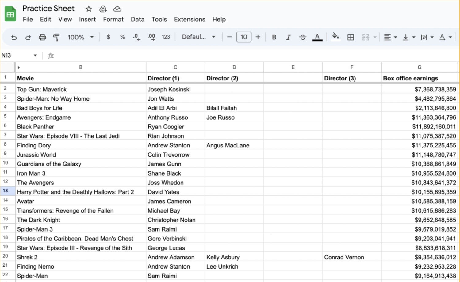
1. Open your Google Sheet.

2. Highlight your data.

3. Go to Insert > Chart.

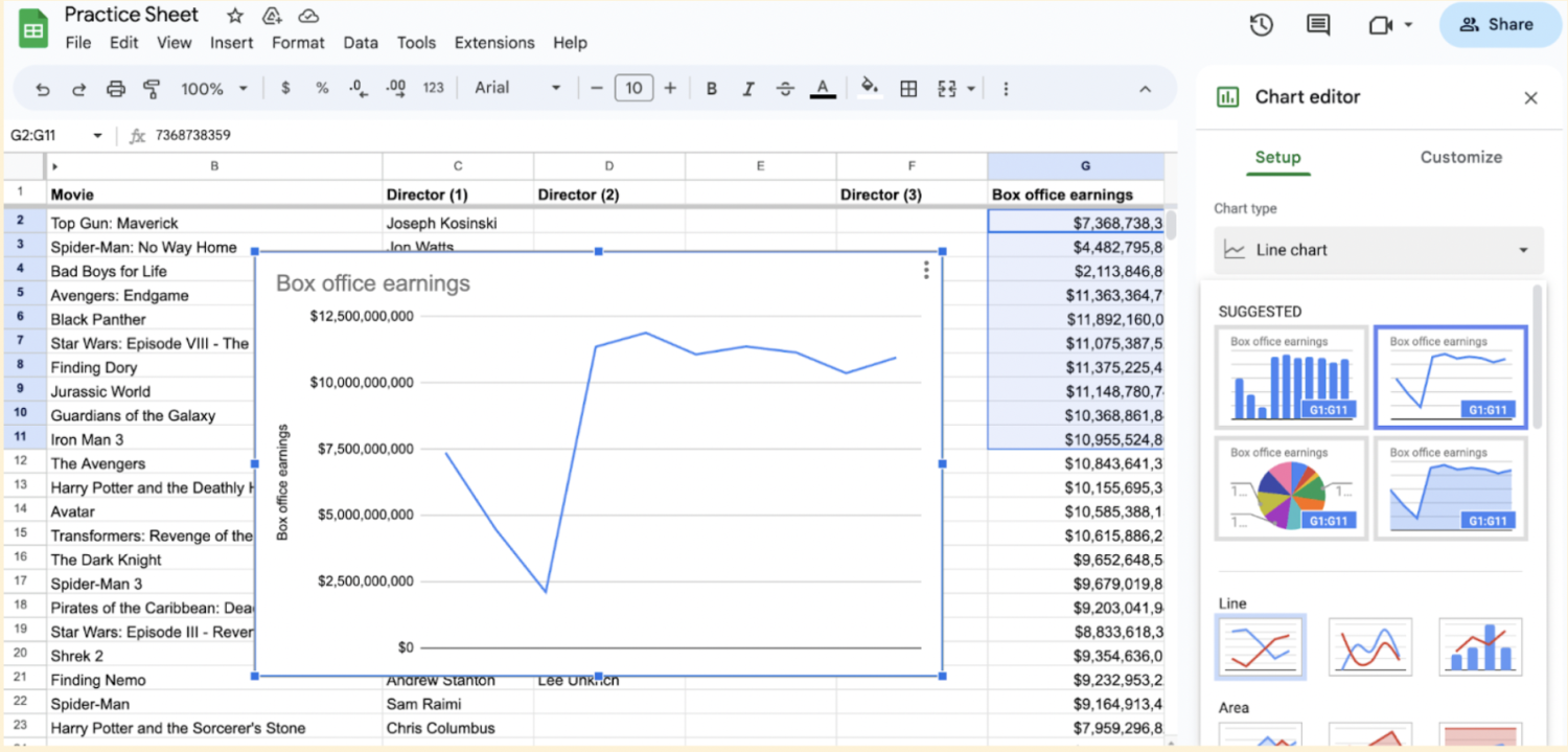
4. Choose a chart type.

5. Go to the chart editor and click Customize > Series.

6. Click on Trendline.

Now, let’s break down each step further so you can utilize this tool with your data effectively.

1. Open Google Sheets.

Begin by opening Google Sheets in your web browser.

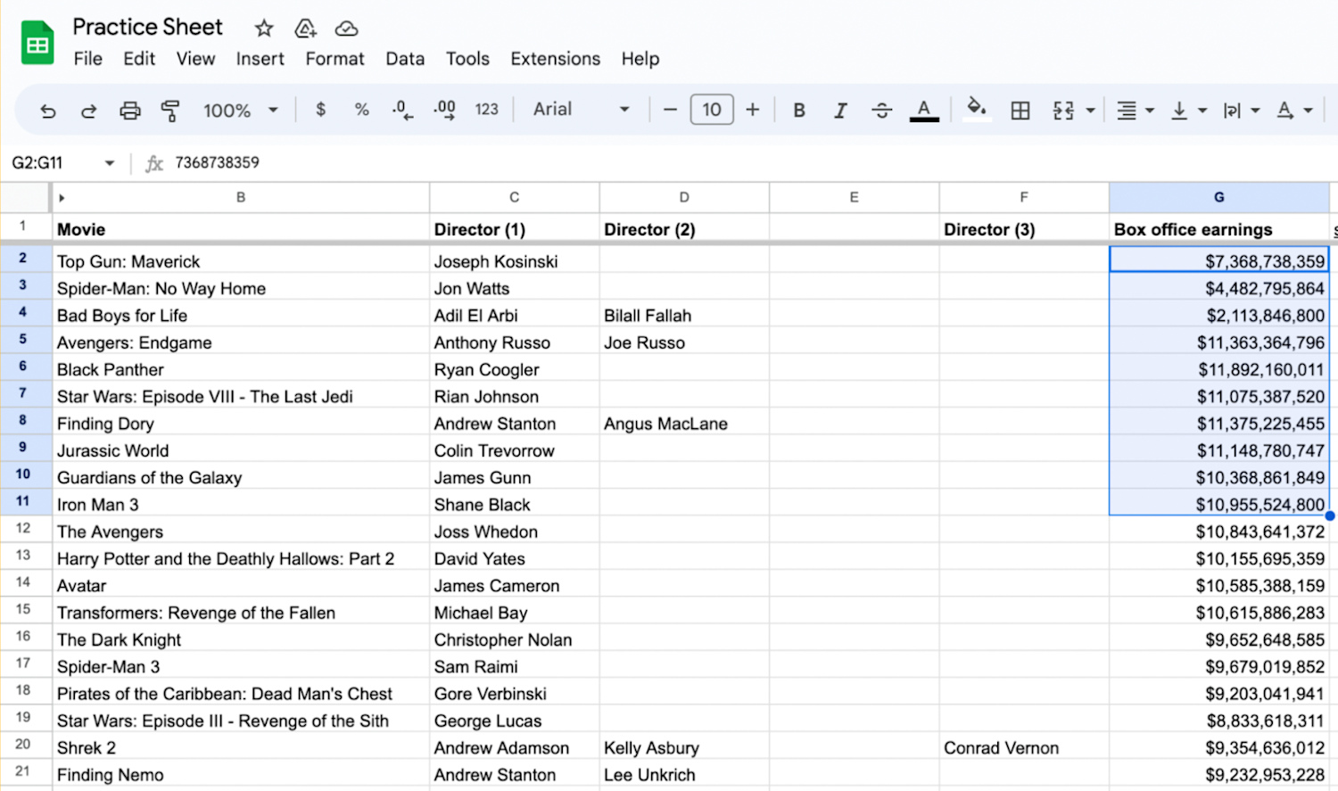
2. Select your data.

Select the data range that you want to include in your chart. Make sure you organize your data in columns or rows.

Read more: Data Trends: Analytics, Governance, and More

3. Go to the “Insert” menu and select “Chart.”

With your data selected, click on the Insert menu at the top and choose Chart. 

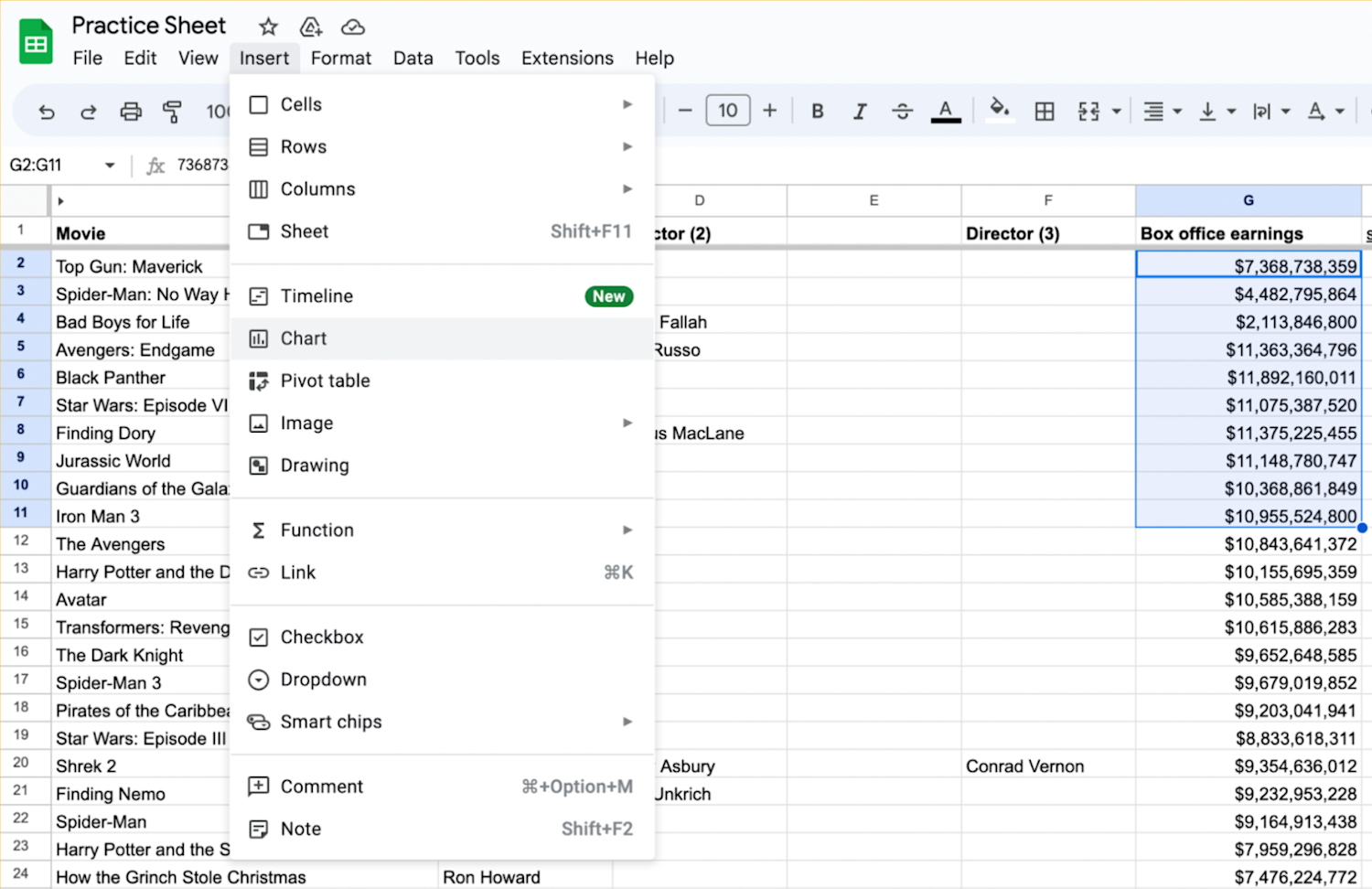
A new window will appear with various chart types to choose from.

4. Select a chart type.

Select the chart type that best represents your data. Common choices for trendline analysis include scatter or line charts. 

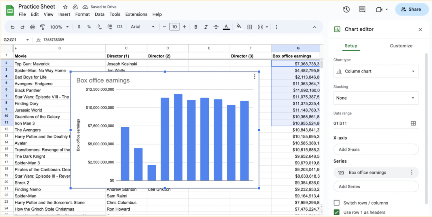
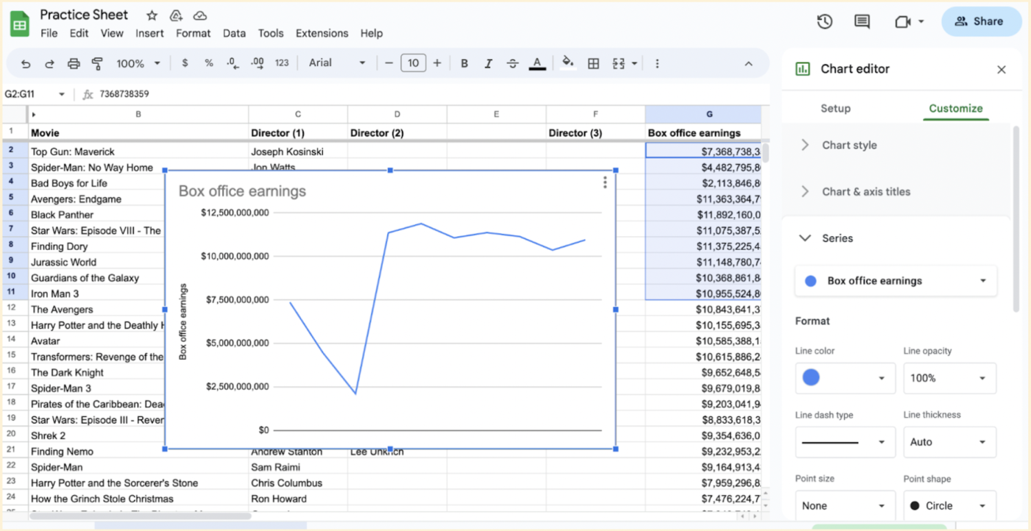
5. Go to the “Customize” tab and select “Series.”

Click on the chart to select it. In the chart editor, click on the Customize tab. Customize your chart as desired. You can change the chart title, axis labels, colors, and other formatting options using the options available in the chart editor.

Scroll down and click on Series.

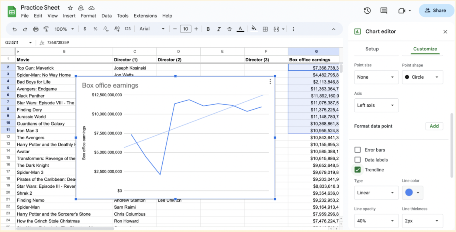
6. Add your trendline.

Tick the Trendline box at the bottom of the Series section.

Best practices with trendlines

When working with trendlines, consider these tips to make the most of your trendline chart:

• Evaluate R-squared value: The R-squared value provides an indication of how well the trendline fits your data. A value close to 1 indicates a strong fit, while a value close to 0 suggests a weak fit. To find this number, check the Show R² box at the bottom of the Series section in the chart editor. 

• Update trendline with new data: If you add or modify data in your sheet, you should continue updating your trendline to reflect any new patterns.

Limitations of trendlines

One limitation of trendlines is that they need to be readjusted as more data is entered. While your trendline may represent the data you have, as new data becomes available, the current trendline may not reflect new information. It is important that you keep trendlines up to date to ensure you are using information that correctly reflects your data.

Treadlines based on highly variable data may also not accurately reflect true information. Trendlines based on more data with less variability will have higher validity on average. When deciding whether to use a trendline, you should consider what type of data you have and whether it can be accurately represented by this type of chart.

How do I add trend arrows in Google Sheets?

Although Google Sheets doesn’t have a built-in feature for inserting trend arrows, you can still add them manually using custom formulas. These trend arrows offer a quick way to spot trends in your data.

For example, consider you have monthly website traffic data for April in Column A and May in Column B, where each row represents the number of visitors for a specific month. To compare the traffic of May with April, apply the following formula to the second cell in Column C:

=IF(B2 > A2, "↑", IF(B2 < A2, "↓", "→"))  

Assuming A1, B1, and C1 are headers and the values start from A2 and B2, cell C2 will return ↑ when May’s traffic rises, ↓ when it falls, and → when the traffic remains the same. Drag this formula down to apply it to other cells in column C. 

You can also go a step further and add custom colors to these arrows using . 

Explore more free resources

Whether you want to do more with spreadsheets or develop your skills, our Career Resources Hub offers an excellent starting point for tutorials, skill assessments, and career planning tools. You might also check out the following: 

• Get another Google Sheets tip: Google Sheets Automation: A Step-by-Step Guide

• Watch a YouTube video: 7 Essential Data Analytics Skills for Beginners

• Hear from an expert: Reimagining Work and Learning with AI: Expert Insights from Dr. Jules White

Accelerate your career growth with a Coursera Plus subscription. When you enroll in either the monthly or annual option, you’ll get access to over 10,000 courses.